The SeaFlux dataset
The SeaFlux data set allows for the homogenization of air-sea CO\(_2\) flux calculations. To minimize the potential differences that may arise during calculation, we’ve made a product available at 1°⨉1° by monthly resolution for 1988-2018. The product can be accessed and downloaded from https://doi.org/10.5281/zenodo.4133802.
Here, we’ll show you how to download the data with Python and quickly calculate air-sea CO\(_2\) fluxes when you only have \(p\)CO\(_2\) based on the bulk flux formulation:
Where \(K_0\) is the solubility of CO\(_2\) in seawater, \(k_w\) is the gas transfer velocity using the formulation of Wanninkhof (1992) that has a square dependence on wind speed (second moment of the wind), \(p\text{CO}_2^{sea}\) is the oceanic partial pressure of carbon dioxide in the surface ocean, \(p\text{CO}_2^{atm}\) is the atmospheric partial pressure of carbon dioxide in the marine boundary layer, \(ice^{free}\) is the fraction of open ocean in a particular grid cell.
Here we tackle the differences that arise in each of these components. In this notebook, we’ll detail how to implement these corrections using Python.
[2]:
%pylab inline

# for the rest of the document seaflux is referred to as sf
import pyseaflux as sf
import xarray as xr
Populating the interactive namespace from numpy and matplotlib
pCO2 area coverage
This correction applies to data-based surface \(p\text{CO}_2^{sea}\) products that provide pseudo-global coverage. However, due to various implementations and predictor variables used by each of these data-based products, there is a difference in the coverage of these products. This is true primarily for the coastal ocean and seasonally ice covered regions.
Recent work by Landschützer et al. (2020) provides a monthly \(p\text{CO}_2^{sea}\) climatology that is available for open ocean, coastal ocean, and seasonally ice-covered seas. By scaling this product, SeaFlux is able to provide a data product that can fill \(p\text{CO}_2^{sea}\) for the pseudo-global data-based products.
For details on this process, please see Fay et al. (2021).
Open example data set
I use the CSIR-ML6 product to demonstrate the data filling procedure. I have pre-downloaded the data into the folder ~/Downloads/.
I use xarray.mfdataset to open the file. This allows for a preprocessor function to be passed. The SeaFlux package includes a preprocess function that tries to conform the data to the SeaFlux data.
[4]:
csir_fname = '~/Downloads/CSIRML6_CO2_19822019_figshare_v2020.6.nc'

preprocessor = sf.data.utils.preprocess()
csir = xr.open_mfdataset(csir_fname, preprocess=preprocessor)

csir_spco2 = csir.spco2
Download scaled climatology
xr.Dataset which provides a useful interface to view the data.Note that the default download location is set to ~/Downloads/SeaFlux_v2021.01. This will create a folder in your downloads folder. This can be changed to any other folder. In addition to downloading the data, a README.txt file will be created in the given directory alongside a downloading log.
[5]:
sf_data = sf.get_seaflux_data(verbose=True)
2021-04-11 16:09:08 [DOWNLOAD]  ================================================================================


2021-04-11 16:09:08 [DOWNLOAD]  Start of logging session
2021-04-11 16:09:08 [DOWNLOAD]  --------------------------------------------------------------------------------
2021-04-11 16:09:08 [DOWNLOAD]    5 files at https://zenodo.org/record/4664653/files/SeaFluxV2021.01_solWeis74.nc
2021-04-11 16:09:08 [DOWNLOAD]  Files will be saved to /Users/luke/Downloads/SeaFlux_v2021.01
2021-04-11 16:09:08 [DOWNLOAD]  retrieving https://zenodo.org/record/4664653/files/SeaFluxV2021.01_solWeis74.nc
2021-04-11 16:09:08 [DOWNLOAD]  retrieving https://zenodo.org/record/4664653/files/SeaFluxV2021.01_icefrac_1988-2018.nc
2021-04-11 16:09:08 [DOWNLOAD]  retrieving https://zenodo.org/record/4664653/files/SeaFluxV2021.01_kwScaled16.5cmhr_1988-2018.nc
2021-04-11 16:09:08 [DOWNLOAD]  retrieving https://zenodo.org/record/4664653/files/SeaFluxV2021.01_pCO2atm_NOAAmbl%2BERA5mslp_1988-2018.nc
2021-04-11 16:09:08 [DOWNLOAD]  retrieving https://zenodo.org/record/4664653/files/SeaFluxV2021.01_spCO2filled_1988-2018.nc
2021-04-11 16:09:08 [DOWNLOAD]  SUMMARY: Retrieved=5, Failed=0 listing failed below:
[7]:
sf_data
[7]:
<xarray.Dataset>
Dimensions:            (lat: 180, lon: 360, product: 6, time: 372, wind: 5)
Coordinates:
  * lat                (lat) float64 -89.5 -88.5 -87.5 -86.5 ... 87.5 88.5 89.5
  * lon                (lon) float64 -179.5 -178.5 -177.5 ... 177.5 178.5 179.5
  * time               (time) datetime64[ns] 1988-01-15 ... 2018-12-15
  * wind               (wind) object 'CCMP2' 'ERA5' 'JRA55' 'NCEP1' 'NCEP2'
  * product            (product) object 'MPI_SOMFFN' 'JMA_MLR' ... 'CSIR_ML6'
Data variables:
    ice                (time, lat, lon) float32 dask.array<chunksize=(372, 180, 360), meta=np.ndarray>
    kw_scaled          (wind, time, lat, lon) float64 dask.array<chunksize=(5, 372, 180, 360), meta=np.ndarray>
    kw_a_scaling       (wind) float64 dask.array<chunksize=(5,), meta=np.ndarray>
    ice_frac           (time, lat, lon) float32 dask.array<chunksize=(372, 180, 360), meta=np.ndarray>
    pCO2atm            (time, lat, lon) float64 dask.array<chunksize=(372, 180, 360), meta=np.ndarray>
    spco2_filled       (product, time, lat, lon) float64 dask.array<chunksize=(6, 372, 180, 360), meta=np.ndarray>
    spco2_clim_scaled  (time, lat, lon) float64 dask.array<chunksize=(372, 180, 360), meta=np.ndarray>
    scaling_factor     (time) float64 dask.array<chunksize=(372,), meta=np.ndarray>
    product_mask       (product, time, lat, lon) bool dask.array<chunksize=(6, 372, 180, 360), meta=np.ndarray>
sol_Weiss74 (time, lat, lon) float64 dask.array<chunksize=(372, 180, 360), meta=np.ndarray>- lat: 180
- lon: 360
- product: 6
- time: 372
- wind: 5
- lat(lat)float64-89.5 -88.5 -87.5 ... 88.5 89.5
- standard_name :
- latitude
- units :
- degrees_north
- axis :
- Y
array([-89.5, -88.5, -87.5, -86.5, -85.5, -84.5, -83.5, -82.5, -81.5, -80.5, -79.5, -78.5, -77.5, -76.5, -75.5, -74.5, -73.5, -72.5, -71.5, -70.5, -69.5, -68.5, -67.5, -66.5, -65.5, -64.5, -63.5, -62.5, -61.5, -60.5, -59.5, -58.5, -57.5, -56.5, -55.5, -54.5, -53.5, -52.5, -51.5, -50.5, -49.5, -48.5, -47.5, -46.5, -45.5, -44.5, -43.5, -42.5, -41.5, -40.5, -39.5, -38.5, -37.5, -36.5, -35.5, -34.5, -33.5, -32.5, -31.5, -30.5, -29.5, -28.5, -27.5, -26.5, -25.5, -24.5, -23.5, -22.5, -21.5, -20.5, -19.5, -18.5, -17.5, -16.5, -15.5, -14.5, -13.5, -12.5, -11.5, -10.5, -9.5, -8.5, -7.5, -6.5, -5.5, -4.5, -3.5, -2.5, -1.5, -0.5, 0.5, 1.5, 2.5, 3.5, 4.5, 5.5, 6.5, 7.5, 8.5, 9.5, 10.5, 11.5, 12.5, 13.5, 14.5, 15.5, 16.5, 17.5, 18.5, 19.5, 20.5, 21.5, 22.5, 23.5, 24.5, 25.5, 26.5, 27.5, 28.5, 29.5, 30.5, 31.5, 32.5, 33.5, 34.5, 35.5, 36.5, 37.5, 38.5, 39.5, 40.5, 41.5, 42.5, 43.5, 44.5, 45.5, 46.5, 47.5, 48.5, 49.5, 50.5, 51.5, 52.5, 53.5, 54.5, 55.5, 56.5, 57.5, 58.5, 59.5, 60.5, 61.5, 62.5, 63.5, 64.5, 65.5, 66.5, 67.5, 68.5, 69.5, 70.5, 71.5, 72.5, 73.5, 74.5, 75.5, 76.5, 77.5, 78.5, 79.5, 80.5, 81.5, 82.5, 83.5, 84.5, 85.5, 86.5, 87.5, 88.5, 89.5]) - lon(lon)float64-179.5 -178.5 ... 178.5 179.5
- standard_name :
- longitude
- units :
- degrees_east
- axis :
- X
array([-179.5, -178.5, -177.5, ..., 177.5, 178.5, 179.5])
- time(time)datetime64[ns]1988-01-15 ... 2018-12-15
array(['1988-01-15T00:00:00.000000000', '1988-02-15T00:00:00.000000000', '1988-03-15T00:00:00.000000000', ..., '2018-10-15T00:00:00.000000000', '2018-11-15T00:00:00.000000000', '2018-12-15T00:00:00.000000000'], dtype='datetime64[ns]') - wind(wind)object'CCMP2' 'ERA5' ... 'NCEP1' 'NCEP2'
array(['CCMP2', 'ERA5', 'JRA55', 'NCEP1', 'NCEP2'], dtype=object)
- product(product)object'MPI_SOMFFN' ... 'CSIR_ML6'
- description :
- Names of the data-based products. See http://www.bgc-jena.mpg.de/SOCOM/Methods.html for more details.
array(['MPI_SOMFFN', 'JMA_MLR', 'JENA_MLS', 'CMEMS_FFNN', 'NIES_FNN',
       'CSIR_ML6'], dtype=object)
- ice(time, lat, lon)float32dask.array<chunksize=(372, 180, 360), meta=np.ndarray>
- unit :
- frac
- description :
- sea ice fraction from OISST
Array Chunk Bytes 96.42 MB 96.42 MB Shape (372, 180, 360) (372, 180, 360) Count 3 Tasks 1 Chunks Type float32 numpy.ndarray - kw_scaled(wind, time, lat, lon)float64dask.array<chunksize=(5, 372, 180, 360), meta=np.ndarray>
- long_name :
- gas transfer velocity for CO2
- units :
- cm/hr
- description :
- k = a * <U2> * Sc660 where a is scaled to a global 14C bomb estimate of 16.5 cm/hr. Note that the global kw is weighted by sea ice cover, thus the mean of kw will not be 16.5 cm/hr. <U2> is the second moment of the wind speed calculated at the native resolutoin of the wind product and then averaged to monthly by 1deg. Sc660 is the Schmidt number for CO2 normalised to 660 as in Wanninkhof (1992): (Sc / 660)^-0.5. For more details on this calculation see Sarmiento and Gruber (2006), Wanninkhof (2014) and Sweeney et al. (2007).
Array Chunk Bytes 964.22 MB 964.22 MB Shape (5, 372, 180, 360) (5, 372, 180, 360) Count 3 Tasks 1 Chunks Type float64 numpy.ndarray - kw_a_scaling(wind)float64dask.array<chunksize=(5,), meta=np.ndarray>
- description :
- scaling parameter $a$ in the equation $k_w = a \cdot U^2_{10} \cdot Sc^{660}$ where $U^2_{10}$ is calculated at the native resolution of $U_{10}$ and then averaged to monthly by 1deg.
- c14bombFlux :
- 16.5
Array Chunk Bytes 40 B 40 B Shape (5,) (5,) Count 3 Tasks 1 Chunks Type float64 numpy.ndarray - ice_frac(time, lat, lon)float32dask.array<chunksize=(372, 180, 360), meta=np.ndarray>
- unit :
- frac
- description :
- sea ice fraction from OISST
Array Chunk Bytes 96.42 MB 96.42 MB Shape (372, 180, 360) (372, 180, 360) Count 3 Tasks 1 Chunks Type float32 numpy.ndarray - pCO2atm(time, lat, lon)float64dask.array<chunksize=(372, 180, 360), meta=np.ndarray>
- units :
- uatm
- description :
- Atmospheric pCO2 for the marine boundary layer is calculated from the NOAAs marine boundary layer pCO2 with: xCO2 * (Patm - pH2O). Patm is the ERA5 mean sea level pressure. pH2O is calculated using vapour pressure from Dickson et al. (2007)
- citation :
- Ed Dlugokencky and Pieter Tans, NOAA/ESRL (www.esrl.noaa.gov/gmd/ccgg/trends/)
Array Chunk Bytes 192.84 MB 192.84 MB Shape (372, 180, 360) (372, 180, 360) Count 3 Tasks 1 Chunks Type float64 numpy.ndarray - spco2_filled(product, time, lat, lon)float64dask.array<chunksize=(6, 372, 180, 360), meta=np.ndarray>
- units :
- uatm
- source :
- http://www.bgc-jena.mpg.de/SOCOM/Methods.html
- description :
- Surface ocean partial pressure of carbon dioxide as estimated with observation-based models. All products have been converted to a monthly 1x1 deg resolution. Only ocean pixels have been preserved using an SST mask. For information on each product and download links see http://www.bgc-jena.mpg.de/SOCOM/Methods.html for more details. All products have been used with permission of the authors.
Array Chunk Bytes 1.16 GB 1.16 GB Shape (6, 372, 180, 360) (6, 372, 180, 360) Count 3 Tasks 1 Chunks Type float64 numpy.ndarray - spco2_clim_scaled(time, lat, lon)float64dask.array<chunksize=(372, 180, 360), meta=np.ndarray>
- units :
- uatm
- long_name :
- scaled climatological surface ocean partial pressure of CO2
- source :
- https://doi.org/10.5194/essd-12-2537-2020
- description :
- Scaled surface ocean pCO2 as estimated using the MPIULB-SOMFFN product (Landschutzer et al. 2020). spco2_clim_scaled is used to fill spco2 producing the spco2_filled variable. Scaling is performed using the `spco2_clim_scaling` variable. Taking `spco2_clim_scaled / spco2_clim_factor` will result in the original climatology.
Array Chunk Bytes 192.84 MB 192.84 MB Shape (372, 180, 360) (372, 180, 360) Count 3 Tasks 1 Chunks Type float64 numpy.ndarray - scaling_factor(time)float64dask.array<chunksize=(372,), meta=np.ndarray>
- units :
- dimensionless
- description :
- Scaling is applied to spco2_climatology that is then used to fill spco2. Scaling factor was estimated as: factor = (spco2_climatology / ensemble).mean(lat, lon) where ensemble is the mean of [MPI_SOMFFN, JMA_MLR, JENA_MLS, CMEMS_FFNN, NIES_FNN, CSIR_ML6] for overlapping regions.
Array Chunk Bytes 2.98 kB 2.98 kB Shape (372,) (372,) Count 3 Tasks 1 Chunks Type float64 numpy.ndarray - product_mask(product, time, lat, lon)booldask.array<chunksize=(6, 372, 180, 360), meta=np.ndarray>
- description :
- A mask that indicates the extent of the original pCO2 product before being filled with `spco2_clim_scaled`.
Array Chunk Bytes 144.63 MB 144.63 MB Shape (6, 372, 180, 360) (6, 372, 180, 360) Count 3 Tasks 1 Chunks Type bool numpy.ndarray - sol_Weiss74(time, lat, lon)float64dask.array<chunksize=(372, 180, 360), meta=np.ndarray>
- description :
- CO2 solubility in seawater using the formulation of Weiss 1974
- units :
- mol/m3/uatm
- long_name :
- CO2 solubility in seawater
Array Chunk Bytes 192.84 MB 192.84 MB Shape (372, 180, 360) (372, 180, 360) Count 3 Tasks 1 Chunks Type float64 numpy.ndarray
Filling the example data
Rather than creating a whole new way of doing things, SeaFlux leverages xarray functionality. The fillna method will fill missing data with the given input, which is exactly what we have to do! For this to work, the dimensions of both data arrays need to be the same, i.e., the time, lat and lon have to have the same values.
[8]:
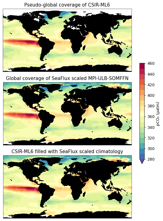
csir_filled = csir_spco2.fillna(sf_data.spco2_clim_scaled)
The figure below shows average pCO2 for the unfilled (CSIR), filler (MPI-ULB-SOMFFN scaled), and filled products (unfilled + filler).
Fluxes
Gas transfer velocity: Here, for the sake of simplicity, we choose to use \(k_w\) that has been calculated with the ERA5 winds only. However, in the product, we have calculated \(k_w\) for the following wind products: CCMP, ERA5, JRA55, NCEP R1/2. The \(k_w\) for this dataset is scaled to a global value of 16.5 cm hr\(^{-1}\) over the period 1988-2017 (30 years). The period is chosen as all wind products overlap.
Solubility: Solubility is calculated using the Weiss (1980) formulation, with the coefficients from the table in Wanninkhof (2014). The other variables used are sea surface temperature and salinity.
Atmospheric pCO2: Atmospheric \(p\text{CO}_2\) for the marine boundary layer is calculated from the NOAAs marine boundary layer \(x\text{CO}_2\) product (https://www.esrl.noaa.gov/gmd/ccgg/trends/): \(x\text{CO}_2 * (P_{atm} - p\text{H}_2\text{O})\). Where \(P_{atm}\) is the ERA5 mean sea level pressure. \(p\text{H}_2\text{O}\) is calculated using vapour pressure from Dickson et al. (2007).
Ice cover and sea surface temperature: We use the NOAA OI.v2 SST monthly fields. These are derived by a linear interpolation of the weekly optimum interpolation (OI) version 2 fields to daily fields then averaging the daily values over a month. The monthly fields are in the same format and spatial resolution as the weekly fields. The ice field shows the approximate monthly average of the ice concentration values input to the SST analysis. Ice concentration is stored as the percentage of area covered. For the ice fields, the land and coast grid cells have been set to the netCDF missing value. (ftp://ftp.cdc.noaa.gov/Datasets/noaa.oisst.v2/)
Salinity: We use the EN4.2.1 salinity for the shallowest level. Specifically, we use the objective analyses data with the Gouretski and Reseghetti (2010) corrections. (https://www.metoffice.gov.uk/hadobs/en4/download-en4-2-1.html)
[10]:
# download flux data - verbosity is False by default
sf_data = sf.data.get_seaflux_data()

ds = sf_data.sel(wind='ERA5').drop('wind')
# use the SeaFlux function to calculate area
ds['area'] = sf.get_area_from_dataset(ds)

# assigning variables and performing unit transformations
kw = ds.kw_scaled * (24/100)      # cm/hr --> m/d
K0 = ds.sol_Weiss74               # mol/m3/uatm
dpco2 = csir_filled - ds.pCO2atm  # uatm
ice_free = 1 - ds.ice.fillna(0)   # fill the open ocean with zeros
area = ds.area                    # m2
[11]:
# bulk flux calculation
flux_mol_m2_day = kw * K0 * dpco2 * ice_free
flux_avg_yr = flux_mol_m2_day.mean('time') * 365  # molC/m2/year
flux_integrated = (flux_mol_m2_day * area * 365 * 12.011).sum(dim=['lat', 'lon'])  # gC/year
Unit analysis
The SeaFlux product provides the remaining parameters to calculate fluxes. This means that the calculation can be a simple multiplication. However, units have to be taken care of. Below we show a table of the units for each of the SeaFlux variables used in the bulk flux calculation.
Variable |
SeaFlux units |
Transformation |
Output units |
|---|---|---|---|
\(\Delta p\text{CO}_2\) |
µatm |
µatm |
|
\(K_0\) |
mol m\(^{-3}\) µatm\(^{-1}\) |
mol m\(^{-3}\) µatm\(^{-1}\) |
|
\(k_w\) |
cm hr\(^{-1}\) |
\(\times \frac{24}{100}\) |
m day\(^{-1}\) |
ice\(^{conc}\) |
ice fraction |
\(1 - ice^{conc}\) |
ice free fraction |
area |
m\(^2\) |
m\(^2\) |
|
BULK FLUXES |
|||
\(F\text{CO}_2\) |
\(K_0 \cdot k_w \cdot \Delta pCO_2 \cdot\) ice |
molC m\(^{-2}\) d\(^{-1}\) |
|
INTEGRATION |
|||
\(F\text{CO}_2^{int}\) |
molC m\(^{-2}\) d\(^{-1}\) |
\(\times\) (m\(^2 \cdot\) 12.01 g mol\(^{-1}\) \(\cdot\) 365 d yr\(^{-1}\)) |
gC yr\(^{-1}\) |
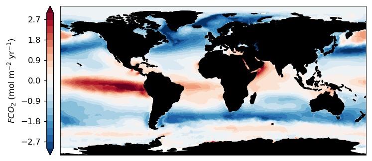
The figure below shows the output for the fluxes calculated using the SeaFlux data. Notice that the ice covered regions, particularly the Arctic, have low air-sea CO\(_2\) fluxes. The output has been multiplied by 365 days/year to convert the flux to \(mol C\ m^{-1}\, yr^{-2}\).
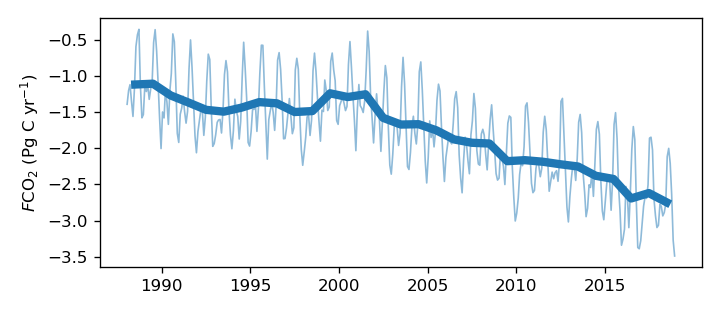
The bottom figure shows the globally integrated air-sea CO\(_2\) fluxes. Here, the fluxes have been multiplied by the area (\(m^2\)) and converted to \(gC\ yr^{-1}\) (using the conversion shown in the table above).